The Ternary Goldbach Conjecture and Vinogradov’s Theorem
For $n \in \Z$, let
$$r_k(n) := \#\lbrace(p_1, p_2, \dots, p_k) \colon p_i \t{ prime, } \sum_{i \leq k} p_i = n\rbrace$$
In June 1742, Christian Goldbach exchanged letters with Leonhard Euler in which his namesake conjectures were formulated.
Conjecture 1 is also known as the strong Goldbach conjecture. Implicit in these letters is a weaker version of the conjectures, which was proved by Helfgott in 2013.
The weak, very weak, and extremely weak conjectures are true. The very strong and extremely strong conjectures are false. The strong conjecture remains open. (Source: xkcd 1310)
Helfgott’s proof of Theorem 2 – although substantially more involved – follows the rough outline of the proof of a result of Vinogradov from the 1930s.
For the lower bound, since $1 - x \geq e^{-2x}$ for small enough $x$, \begin{align} \mathfrak{S}(n) \geq \prod_p \paren{1 - \f{1}{(p-1)^2}} \gg \prod_p e^{\f{-1}{2(p-1)^2}} \geq e^{-\sum_{n \in \NN} \f{1}{n^2}} = e^{-\zeta(2)}.\nonumber \end{align} $\Box$
Fixing $A$, we see that for large enough $n$, $r_3(n) > 1$ and the ternary Goldbach conjecture holds. Unfortunately, the implicit constant in the asymptotic is ineffective due to the use of Siegel’s theorem (on elliptic curves) in the proof, so Theorem 3 is inamenable to explicit bounds. This means that we cannot use this method to find an $N$ beyond which $r(n) > 0$.
This post is based on a talk I gave at the No Theory seminar at UChicago in Winter 2023, following discussions I had with Timothy Ngotiaoco. I will explicate the circle method and how it may be applied to this problem, focusing mainly on the setup of the proof (before the walls of inequalities begin). I am sure that everything I write here is well known, but I was not able to find it (and in particular, Lemma 6) written down in detail anywhere. As such, please let me know if you see any errors.
Expressing the count as an integral
Vinogradov proved Theorem 3 using the circle method.
A common strategy in analytic number theory is – given a function $f \colon \NN \rightarrow \C^{\times}$ of interest – to study the associated Dirichlet series $$F(s) := \sum_{n \in \NN} f(n)n^{-s}.$$
We can then apply complex analytic methods to conclude properties of $f$ from analytic properties of $F$. For example, Ikehara’s Tauberian theorems can be used to obtain asymptotic bounds on $\sum_{n \leq N} f(n)$ based on the residue of $F$ at $s = 1$.
The circle method is similar, but more Fourier analytic. The Fourier transform of $f \colon \ZZ \rightarrow \C^{\times}$ is
$$\hat{f}(\theta) := \sum_{n \in \ZZ} f(n)e(-n\theta),$$
where for $\theta \in \R/\Z$, $e(n\theta) := e^{2\pi i n \theta}$. We can recover the coefficients from $\hat{f}(\theta)$ using inverse Fourier transform,
$$f(n) = \int_{\theta \in \R/\Z} \hat{f}(\theta)e(n\theta) d\theta.$$
Suppose that $f(n)$ is the indicator function for prime numbers. Then, $$\hat{f}(\theta)^3 = \sum_{n \in \ZZ} \paren{\sum_{a + b + c = n} f(a)f(b)f(c)}e(-n\theta) = \sum_{n \in \ZZ} r(n)e(-n\theta).$$
Therefore, we have $$r(n) = \int_{\theta \in \R/\Z} \hat{f}(\theta)^3.$$
For our application, it will be convenient to replace $f(n)$ with the von Mangoldt function $\Lambda(n)$, defined as
$$\Lambda(n) := \begin{cases} \log p & n = p^k \t{ for some prime } p \\ 0 & \t{otherwise}. \end{cases}$$
As we will see shortly, we will need to work with truncated sums rather than power series to avoid convergence issues. Thus, writing $$S(\theta) := S_N(\theta) = \sum_{n \leq N} \Lambda(n)e(-n\theta),$$ we observe that the coefficient of $e(n\theta)$ in $S(\theta)^3$ counts the number of ways to express $n$ as a sum of three prime powers not exceeding $N$. Our integral of interest is then
\begin{equation} \int_{\theta \in \R/\Z} S(\theta)^3e(n\theta). \end{equation}
Remark: The von Mangoldt function is a common stand-in for the prime indicator function in analytic number theory. For example, many proofs of the prime number theorem, rather than showing that $\pi(x) := \sum_{n \leq x} f(n) \sim \f{x}{\log x}$ directly, instead prove that $\psi(x) := \sum_{n \leq x} \Lambda(n) \sim x$. These two are equivalent – roughly each prime up to $x$ is counted $\f{\log x}{\log p}$ times, with weight $\log p$, so if there are $\f{x}{\log x}$ primes then the sum ought to be $x$. This connects nicely to the Riemann zeta function, because $$\f{\zeta’(s)}{\zeta(s)} = \sum_{n \in \NN} \Lambda(n)n^{-s},$$ and allows us to relate the distribution of prime numbers to the analytic behavior of $\zeta(s)$.
Remark: The circle method, usually called the Hardy-Littlewood circle method, had its beginnings in work by Hardy and Ramanujan on the asymptotics of the partition function. Its utility was expanded significantly by work of Hardy and Littlewood, who applied it to counting the number of ways to express numbers as sums of $k^{th}$ powers (Waring’s problem). The circle method is thus a partial example of Stigler’s law of eponymy.
Singularities on the unit circle
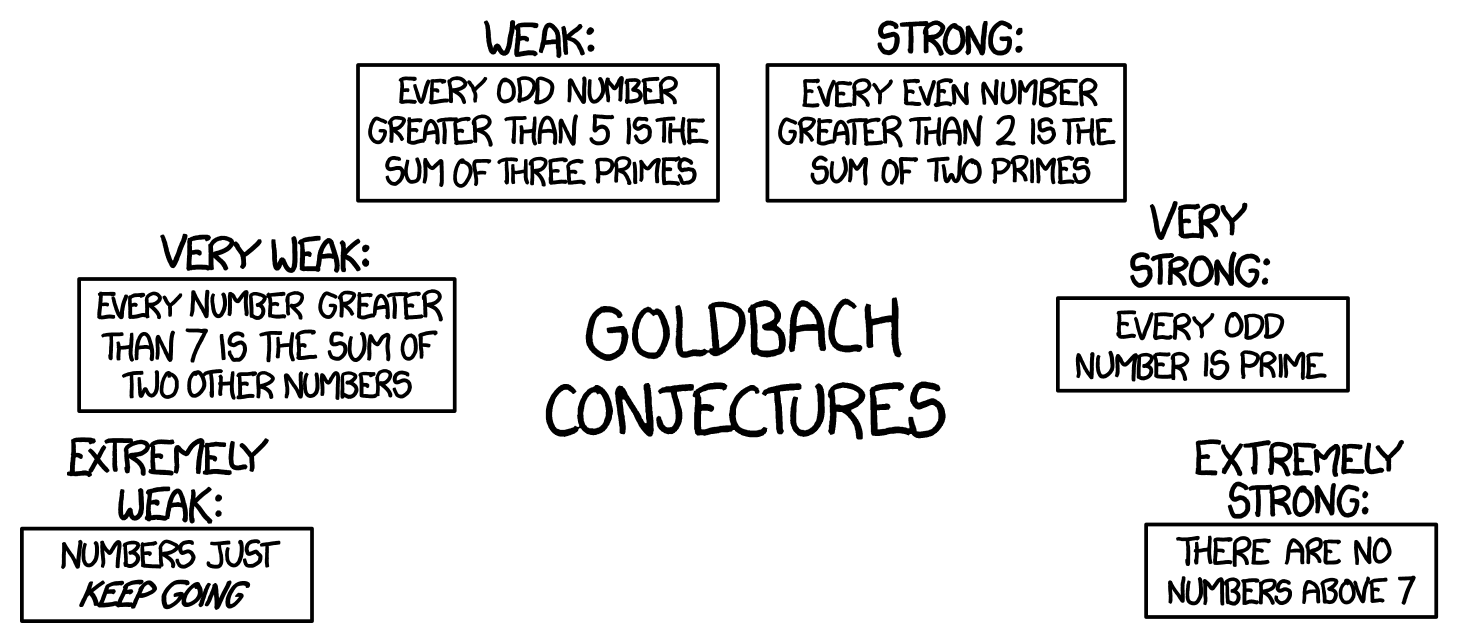
The problem of studying $r(n)$ now reduces to studying the integral in Equation 1. We will break it up into an integral over major arcs – regions where the integrand is large but well estimable – and minor arcs – where the integrand is small but may be difficult to control. The major arcs will give us the main term and the minor arcs will give us the error term. To get a sense of how to choose the major and minor arcs, let’s do some graphing. Abusing notation, we write $S_N(z) := \sum_{n \leq N} \Lambda(n)z^n$.
$S_{2500}(z)^3$ on the unit disk.
Remark: Here’s a quick crash course if you haven’t thought about plots of complex functions too hard before. Given a complex-valued function $f$, if $f(z)$ is $(r,\theta)$ in polar coordinates, then the hue of the graph of $f$ at the point $z$ tells us about $\theta$ and the brightness at $z$ tells us about $r$. Precisely, ROYGBIV corresponds to $\theta = [0, 2\pi)$, larger magnitudes are closer to white, and smaller magnitudes are closer to black. Zeroes look locally like $z^k$, so we expect to see the colors ROYGBIV as we go clockwise around a zero. Poles look locally like $z^{-k}$, so we expect to see the colors in the opposite order around a pole. Intuitively, the “worse” a singularity is, the greater the distortion around it ought to be.
As expected, we see a large black patch in the middle since $S_N(z)$ is small near $z = 0$. We are interested in the behavior of $S_N(z)^3$ along the unit circle, so we should focus on the boundaries of the disk. It’s a little bit difficult to see what’s happening, so to simplify things, let’s plot $S_N(z)$ instead of its cube.
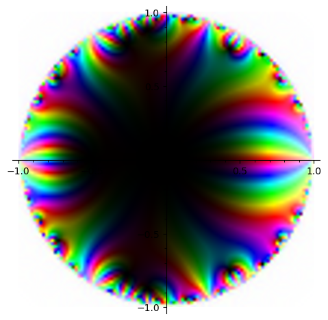
$S_{7500}(z)$ on the unit disk. The dots around the outside mark the points $e^{2\pi i \theta}$ for $\theta \in \Q \cap [0,1)$ with denominators at most $7$. Dots with the same denominator are the same shade of grey.
Following the remark, $S_N(z)$ appears to have a large singularity at $\theta = 0$, a smaller singularity at $\f{1}{2}$, and increasingly small singularities when the denominator is $3$, $5$, or $7$. When the denominator is $6$, we see a larger-than-expected singularity, and when the denominator is $4$ there appears to be no singularity (or a very small one). Before we explain this, we need the following preliminary lemma, whose proof we leave as an exercise.
At least heuristically, this tells us that the “badness” of the singularity at an $s^{\t{th}}$ root of unity should be proportional to $\f{\mu(s)}{\phi(s)}$. There are ways to make statements vaguely like this precise, but I haven’t really thought about whether it can be done here.
This helps explains the observations we made earlier. There is a singularity at every $s \in \Q$. If $s = \f{a}{p}$ for a prime $p$, Lemma 6 tells us that the “badness” of the singularity decreases as $p$ increases. There is no contribution from $s = 4$ because $\mu(4) = 0$. The contribution from $s = 6$ is unexpectedly large because $\phi(6) < \phi(5)$. We have the lower bound $\phi(s) \geq \f{s}{(e^{\gamma} + o(1))\log \log s}$, so we expect the largest contributions to come near $s \in \Q$ with small denominators.
Remark: Lemma 6 tells us that the series $\sum_{n \in \NN} \Lambda(n)z^n$ has a singularity whenever $z$ is a $m^{\t{th}}$ root of unity for $m$ squarefree. The set of numbers with squarefree denominator is dense in $\R/\Z$, so this implies that the series has singularities everywhere on the unit circle! This also follows from the Hadamard-Ostrowski theorem, which says that power series with sufficient gaps between nonzero coefficients cannot be analytically continued beyond their radius of convergence. In some sense, the fact that there are singularities everywhere has more to do with the gaps between nonzero coefficients in this sequence than to the precise distribution. However, the relative weighting of the singularities in our series depends on the distribution.
Fix $P := (\log N)^B$ and $Q = N(\log N)^{-B}$, for $B$ to be chosen later (in terms of $A$). For any $m \leq P$ and $a \in \lbrace0, 1, \dots, m-1\rbrace$ such that $(a, m) \equiv 1$, we define the major arc $$\mathfrak{M}(a,m) := \lbrace\theta \in \R/\Z \colon |\theta - \f{a}{m}| \leq \f{1}{Q}\rbrace.$$
Observe that $\mathfrak{M}(a,m) \cap \mathfrak{M}(a’, m’) = \emptyset$ unless $m = m’$ and $a = a’$, since $$\abs{\f{a}{m} - \f{a’}{m’}} = \abs{\f{am’ - a’m}{mm’}} \geq \f{1}{mm’} \geq \f{1}{P^2} \geq \f{1}{Q}.$$
The major arcs are then $\cup_{a, m} \mathfrak{M}(a, m)$ and the minor arcs are their complement in $\R/\Z$. Now that we have chosen the major and minor arcs, the goal is to bound the integral on each part. I may post about the main body of the proof in the future, but until then refer readers to Chapter 26 of Davenports Multiplicative Number Theory.